The first thing anyone learns about game theory is typically the prisoner’s dilemma. Individual rationality leads to an outcome that leaves everyone worse off. The second thing anyone learns about game theory is typically that, with a high enough value toward future payoffs, cooperation in the prisoner’s dilemma is possible if the game is repeated infinitely.
This week, we had an interesting problem in an assignment for a game theory course I’m currently taking. Thanks to the help of my colleagues, we were able to solve it mathematically, but I wanted to test out simulating the problem in code, which is what led to this post.
The problem consists of a modified infinitely repeated Prisoner’s Dilemma, where if a player choose to cooperate, her realized action might not actually be to cooperate: the realized action will be to cooperate with probability $p$ and to defect with probability $1-p$. If a player chooses to defect, the realized action will certainly be to defect. The payoff matrix is as follows:
| C | D | |
|---|---|---|
| C | $\omega, \omega$ | $0, \omega+r$ |
| D | $\omega+r, 0$ | $r,r$ |
Players discount at a rate of $\delta$, and $\omega > r > 0$.
Let’s consider how we might model a 2-period trigger strategy using simulations, this time in R.
omega <- 2
r <- 1
delta <- 1/2
sims <- 1000
rounds <- 100
We begin by parameterizing the game, this is fairly straightforward. The two values we are not parameterizing are p, which we will change inside the code, and the number of periods in the trigger strategy. If anyone has any suggestions on how to pull this off without using Bellman equations and giving away the mathematical part of the homework) please let me know in the comments. Anyways, in this case, we will play for 100 rounds, simulating the game 1000 times.
storevalue_1 <- list()

for(i in 1:sims) {

round <- 1
round_outcome <- list()
value_1 <- list()
Now, we start the loop over the number of desired simulations, and create objects to store the outputs. I know this isn’t great practice in R, but I’ve been going back and forth between R and Python and have gotten my syntax a bit jumbled up. Note that we define round as 1, we will add to this as the loop continues.
while(round < rounds) {
  round_outcome[round] <- sample(c("cooperate-cooperate", "cooperate-defect", "defect-cooperate", "defect-defect"), 1)
While the round object is less than rounds, the specified number of rounds to play, we sample from the four possible outcomes. Since we are playing a trigger strategy, we assume that both players will start off wanting to cooperate, but since p = 1/2, this will only occur 1/4 of the time. Then the simulation begins to branch:
  if (round_outcome[round] == "cooperate-cooperate") {
    value_1[round] <- omega
    round <- round + 1
In this first case, both players successfully cooperated, and both players get ω, and we add 1 to the round ticker. Note that since the game is symmetric, we only have to specify player 1’s payoffs.
  } else if (round_outcome[round] == "cooperate-defect") {
    value_1[round] <- 0
    round <- round + 1
    value_1[round] <- r
    round <- round + 1
    value_1[round] <- r
    round <- round + 1
Here, player 1’s realized action was to cooperate, but player 2 defected. Player 1 gets 0, and we enter into a two-period punishment phase, where both players get r for two periods.
  } else if (round_outcome[round] == "defect-cooperate") {
    value_1[round] <- omega+r
    round <- round + 1
    value_1[round] <- r
    round <- round + 1
    value_1[round] <- r
    round <- round + 1
Now, player 1 is the one whose realized action was to defect, while player 2 cooperated. Player 1 will get ω+r, and the game enters the two-period punishment phase.
  } else {
    value_1[round] <- r
    round <- round + 1
    value_1[round] <- r
    round <- round + 1
    value_1[round] <- r
    round <- round + 1
  }
}
Finally, the last possibility is when both player’s realized actions are to defect, and so both players earn r, and we enter the two-period punishment phase.
storevalue_1[[i]] <- value_1
}
We can now store player 1’s values for each round and repeat the simulation 1000 times.
index_1 <- lapply(1:(rounds-3), function(x) sapply(1:sims, function(i) mean(storevalue_1[[i]][[x]])))

payoff_1 <- sapply(1:(rounds-3), function(x) mean(index_1[[x]])*delta^(x-1))

data_1 <- cbind.data.frame(1:(rounds-3), payoff_1)
names(data_1) <- c("round", "payoff")
Here we take the expected value of the payoffs at each round for all of the simulations and store things neatly in a dataframe.
And we’re all done!
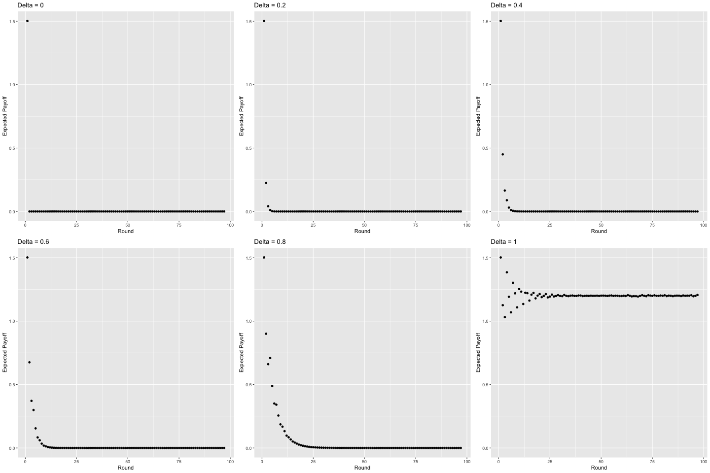
As an added bonus, I took the liberty of using gganimate to show what happens as you vary the discount factor from 0 to 1 by 0.01 each time, shown below.

Interestingly, with sufficiently high discounting ($\delta$ ≈ 0.75), players start to value some of the later rounds more than the earlier rounds and the curve becomes “jagged” as opposed to strictly decreasing given that in expectation, there is a higher probability of exiting a punishment phase in some of these rounds and we value the future enough for this to matter. For example, consider $\delta$ = 1. In the first round, players will earn a payoff of approximately 1.50 in expectation. In the second round they earn around 1.13, in the third, around 1.03, but then in the fourth, 1.39. This logic plays out for later rounds as well (the 5th, 6th, 7th, 8th, 9th, and 10th rounds yield players 1.19, 1.07, 1.30, 1.22, 1.10, and 1.25 in expectation, respectively). You can show this mathematically, but I’m not going to do so becaues then I’d be giving away the answers to my homework.
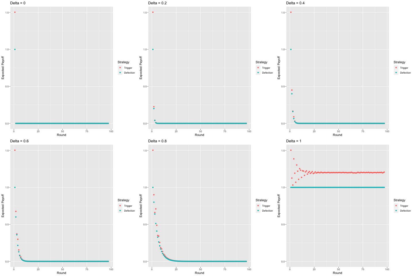
Finally, I present a comparison of the two-period trigger strategy with pure defection, again, varying the discount factor.
