This week’s Riddler Classic is about what happens when you randomly chop up a ruler into four different pieces.
Edit: this solution was mentioned in the article describing the answer! You can read the write-up here.
Here’s the text of the puzzle, and my solution below.
The Riddler Manufacturing Company makes all sorts of mathematical tools: compasses, protractors, slide rules — you name it!
Recently, there was an issue with the production of foot-long rulers. It seems that each ruler was accidentally sliced at three random points along the ruler, resulting in four pieces. Looking on the bright side, that means there are now four times as many rulers — they just happen to have different lengths.
On average, how long are the pieces that contain the 6-inch mark?
The average length of the pieces that contain the 6-inch mark is $\frac{45}{8}$ or 5.625. As usual, I used Monte Carlo simulations to evaluate the problem, so I’ll walk through what I did to find the solution. For this problem, I used R.
First, a simple set-up of a random number seed for reproducibility and designating the number of desired simulations—here 1 million.
set.seed(08162020)
sims <- 10^6
This following line of code simulates the cuts. It creates a $3 \times S$ matrix, where $S$ represents the number of simulations. Each column of the matrix contains three random draws from a uniform distribution with a minimum value of 0 and a maximum value of 12, sorted from smallest to largest. Thus the first row of each column is the placement of the first cut, and so on.
cuts <- sapply(1:sims, function (i) sort(runif(3, 0, 12)))
I then write a simple function to determine in which piece the 6-inch mark falls in. If the first cut (recall these were sorted from smallest to largest) is greater than or equal to 6, then the mark falls inside the first piece. Symmetrically, if the last cut is less than or equal to 6, then the mark falls inside the last piece. These two pieces are the “end” pieces. In the interval between those pieces, the mark is in the second piece if it lies between the first and second cut, and the mark is in the third piece if it lies between the second and third cut. I call these the “middle” pieces.
mark_function <- function(cut) {
  if (cut[1] >= 6) {
    mark <- 1
  }
  else if (cut[3] <= 6) {
    mark <- 4
  }
  else if (cut[1] <= 6 & 6 <= cut[2]) {
    mark <- 2
  }
  else if (cut[2] <= 6 & 6 <= cut[3]) {
    mark <- 3
  }
  return(mark)
}
I then apply the function over each column of the cuts matrix and store which piece contained the mark into a vector of length $S$ called marks.
marks <- apply(cuts, 2, mark_function)
Next, I determine the length of each of the key piece with a new function. If the mark is in the first piece then naturally its length is just the location of the first cut. Analogously, if the mark is in the last piece, then its length is the difference between the end of the ruler and the location of the last cut. The length of the piece in the middle interval is the difference between the second and first cut and the third and second cut, respectively.
length_function <- function(cut, mark) {
  if (mark == 1) {
    length <- cut[1] - 0
  }
  else if (mark == 4) {
    length <- 12 - cut[3]
  }
  else if (mark == 2) {
    length <- cut[2] - cut[1]
  }
  else if (mark == 3) {
    length <- cut[3] - cut[2]
  }
  return(length)
}
Applying that function to the columns of the cuts matrix with the values from the marks vector gives another $S$-length vector of the length of the pieces that contain the mark. This is stored into the lengths object.
lengths <- sapply(1:sims, function(i) length_function(cuts[,i], marks[i]))
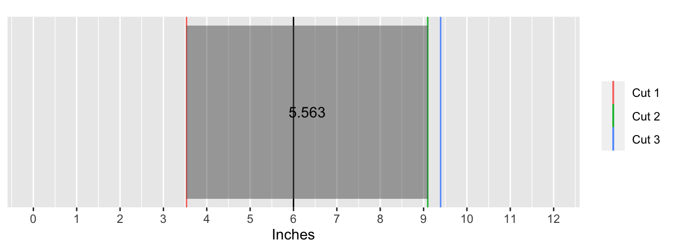
The following animation shows what this process looks like for the first 100 simulations:
Taking the mean of the lengths object yields the answer:
mean(lengths)
As usual with The Riddler, there are still a lot of interesting aspects of the problem to explore besides the answer. A quick peek at the density plot for the lengths of the segments containing the mark is enough to pique one’s curiosity.
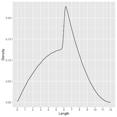
As you might intuit, this curious empirical distribution is a result of mashing the results from the “ends” pieces that contain the mark and the “middle” pieces that contain the mark. The end pieces that contain the mark are longer on average—7.5 inches—than the middle pieces that contain the mark—5 inches. However, the mark does not fall into each type of piece with the same frequency. It falls into the end pieces $\frac{1}{4}$ of the time and falls into the middle pieces for the remaining $\frac{3}{4}$. Of course then, $(\frac{1}{4} \times 5) + (\frac{3}{4} \times \frac{15}{2}) = \frac{45}{8}$.
So when the mark does fall into an end piece, it must have a minimum length of 6 inches, while when considering the middle pieces the lengths can vary more widely—though the distribution is intriguingly asymmetrical. The following image illustrates this by splitting a single histogram into two separate graphs for each of these two types of pieces.

That’s all I have for now, but I’ll include the full set of code below if you’d like to reproduce my analysis or make new plots.
set.seed(08162020)

sims <- 10^6

cuts <- sapply(1:sims, function (i) sort(runif(3, 0, 12)))

mark_function <- function(cut) {
  if (cut[1] >= 6) {
    mark <- 1
  }
  else if (cut[3] <= 6) {
    mark <- 4
  }
  else if (cut[1] <= 6 & 6 <= cut[2]) {
    mark <- 2
  }
  else if (cut[2] <= 6 & 6 <= cut[3]) {
    mark <- 3
  }
  return(mark)
}

marks <- apply(cuts, 2, mark_function)

length_function <- function(cut, mark) {
  if (mark == 1) {
    length <- cut[1] - 0
  }
  else if (mark == 4) {
    length <- 12 - cut[3]
  }
  else if (mark == 2) {
    length <- cut[2] - cut[1]
  }
  else if (mark == 3) {
    length <- cut[3] - cut[2]
  }
  return(length)
}

lengths <- sapply(1:sims, function(i) length_function(cuts[,i], marks[i]))

mean(lengths)

sim_summary <- data.frame(t(cuts))
names(sim_summary) <- c("cut1", "cut2", "cut3")

library(dplyr)

sim_summary <- sim_summary %>%
  mutate(mark = marks,
         piece = case_when(
           mark == 1 | mark == 4 ~ "End Pieces",
           mark == 2 | mark == 3 ~ "Middle Pieces",
         ),
         length = lengths,
         rect_min = case_when(
           mark == 1 ~ 0,
           mark == 2 ~ cut1,
           mark == 3 ~ cut2,
           mark == 4 ~ cut3),
         rect_max = rect_min + length,
         rect_mid = (rect_min + rect_max)/2
  )

library(ggplot2)

ggplot(sim_summary, aes(x = length)) +
  geom_density() +
  scale_x_continuous(limits = c(0, 12), breaks = 0:12) +
  xlab('Length') +
  ylab('Density')

sim_summary %>%
  group_by(mark) %>%
  summarize(mean = mean(length, na.rm=TRUE))

piece_means <- sim_summary %>%
  group_by(piece) %>%
  summarize(mean = mean(length, na.rm=TRUE))

ggplot(sim_summary, aes(x = length)) +
  geom_histogram(bins = 24, alpha = 0.8) +
  scale_x_continuous(limits = c(0, 12), breaks = 0:12) +
  xlab('Length') +
  ylab('Frequency') +
  facet_wrap(~ piece) +
  geom_vline(aes(xintercept = mean), data = piece_means, linetype = "dotted")
I made the animation by placing code to create a plot into a for loop and rendering it in R Markdown with gifski:
```{r, animation.hook="gifski"}
library(gifski)
library(igraph)

for (g in 1:100) {

print(ggplot() +
  geom_vline(aes(xintercept = 6)) +
  geom_vline(aes(xintercept = sim_summary$cut1[g], color = "Cut 1")) +
  geom_vline(aes(xintercept = sim_summary$cut2[g], color = "Cut 2")) +
  geom_vline(aes(xintercept = sim_summary$cut3[g], color = "Cut 3")) +
  geom_rect(aes(xmin = sim_summary$rect_min[g], xmax = sim_summary$rect_max[g], ymin = 0, ymax = 1), alpha = 0.5) +
  geom_text(aes(x = sim_summary$rect_mid[g], y = 0.5, label = round(sim_summary$length[g], 3))) +
  scale_x_continuous(limits = c(0, 12), breaks = 0:12) +
  xlab('Inches') +
  scale_y_continuous(breaks = NULL) +
  coord_fixed(ratio = 4) +
  theme(legend.title = element_blank(),
        axis.title.y = element_blank(),
        axis.text.y = element_blank(),
        axis.ticks.y = element_blank()))

}
```
comments powered by Disqus