The simple game Lingo Wordle has taken the Worldle world by storm. I love word puzzles, so naturally, I’m a big fan. Much has been said about attempts to solve Wordle, typically by people who are much smarter1 than me (e.g., Laurent Lessard, 3Blue1Brown, and Jonathan Olson)—so I won’t pretend to present an optimal solution for the entire game, but I just wanted to share my approach at finding a good starter. Indeed this greedy approach to the first round is unlikely to find the optimal solution since it doesn’t look any further down the line,2 but my computational costs are already quite high and would only blow up taking this any further, so I’ll leave this here for now, since this was a fun exercise.
My idea for a heuristic to find a good first word to guess in wordle is to pick the word maximizes the number of answers that are eliminated after you have selected that first word. In other words (pun intended), what word takes the biggest step to narrow in on the true answer. In the extreme, imagine a word that leaves only 1 remaining word as the possible solution. That’s a great first guess. On the other hand, a word that eliminates no possible solutions is a bad first guess.
To see what word does that for us, we’ll start by defining a function called wordle_round that evaluates this for a single word and a single answer. If the solution is “MORAL”, for example, how many words does guessing “MAPLE” eliminate?
The function takes in as inputs a guess, your guess, the solution solution and a vector of possible solutions, possible_solutions, and starts by splitting the guess into separate characters.
Before we start with the function, though, we’ll download the possible words to guess and the possible solutions, nicely compiled for us by FiveThirtyEight’s The Riddler. Careful with those links, as you may spoil future answers for yourself! Note that these correspond to the solutions when Wordle was run by its original creator, prior to the takeover by the New York Times (and their removal of certain words as possible guesses and answers). We’ll then load these into R as vectors with the read_csv and pull functions.
library("parallel")
library("tidyverse")

possible_solutions <- pull(read_csv("Wordle _ Mystery Words - Sheet1.csv"))
possible_guesses <- pull(read_csv("Wordle _ Guessable Words - Sheet1.csv"))

wordle_round <- function(guess, solution, possible_solutions) {

	guess_split <- unlist(str_split(guess, "", nchar(guess)))
Our next step, then, is to identify how the guess will do given the answer. Which letters will turn black? Green? Yellow?
To assess which letters are black, we’ll check for each possible letter in our guess whether it exists in the solution, and then retain only the letters which are not found in the solution. For our running example, “P” and “E” are black letters.
	black_letters <- sapply(guess_split, function(i)
	    !str_detect(solution, i)
	  )

	black_letters <- names(black_letters[black_letters == TRUE])
Now, we can eliminate any words which have these letters from the possible solution set (as well as the guess). We started with 2,315 possible solutions, and this move gets us down to just 1,058. Not bad, but we still have more words to eliminate.
	possible_solutions <- setdiff(possible_solutions, guess)

	  for (letter in black_letters) {
	    possible_solutions <- possible_solutions[!str_detect(possible_solutions, letter)]
	  }
We now turn to green and yellow letters. We’ll combine these for reasons that will hopefully be made clear later. Green and yellow letters are a little bit more complex, since we can’t just see whether or not the letter occurs in the word, we need to ascertain its position. To do this, for each letter in the guess, we’ll check whether it occurs in the solution and if it occurs in the same position as in the solution using regular expressions. These lines of code return a named logical vector. Its values are equal to TRUE when the solution and letter are in the same place, and FALSE otherwise. Ergo, TRUE values are green, and FALSE values are yellow. It’s names tell us which letter and what position this corresponds to.
	green_yellow_letters <- lapply(1:nchar(guess), function(i)
	    sapply(guess_split, function(j)
	      str_detect(solution, paste0("^", paste(rep(".", i-1), collapse = ""), j))
	    )
	  )

	  green_yellow_letters <- lapply(1:length(green_yellow_letters), function(i)
	    which(green_yellow_letters[[i]] == TRUE)  == i
	  )

	  names(green_yellow_letters) <- sapply(1:length(green_yellow_letters), function(i) i)

	  green_yellow_letters <- unlist(green_yellow_letters)
So for our “MORAL” and “MAPLE” example we get:
1.m   4.a   5.l
TRUE FALSE FALSE
We can then back out what we really want, a list of all the green and yellow letters with their corresponding positions, very easily:
	green_letters <- green_yellow_letters[green_yellow_letters == TRUE]
	green_letters <- str_split(names(green_letters), "\\.")

	yellow_letters <- green_yellow_letters[green_yellow_letters == FALSE]
	yellow_letters <- str_split(names(yellow_letters), "\\.")
This results in:
> green_letters
[[1]]
[1] "1" "m"

> yellow_letters
[[1]]
[1] "4" "a"

[[2]]
[1] "5" "l"
We can now move on to eliminating words, starting with the green matches. We want to keep any remaining words in the set of possible solutions that start with “M”. This block of code will do just that more generally, first finding the words that match the green letters and their positions, and then keeping only those that match from the reduced set of possible solutions.
	if (length(green_letters) != 0) {

	  green_matches <- lapply(1:length(green_letters), function(i)
	    possible_solutions[str_detect(possible_solutions,
	                                  paste0("^", paste(rep(".", as.numeric(green_letters[[i]][1])-1), collapse = ""),
	                                         green_letters[[i]][2]
	                                  ))]
	  )

	  possible_solutions <- intersect(possible_solutions, Reduce(intersect, green_matches))

}
We can do something quite similar for the yellow letters:
	if (length(yellow_letters) != 0) {

	    yellow_matches <- lapply(1:length(yellow_letters), function(i)
	      possible_solutions[str_detect(possible_solutions, yellow_letters[[i]][2])]
	    )

	    possible_solutions <- intersect(possible_solutions, Reduce(intersect, yellow_matches))

	  }
Finally we are left with just six possible solutions!
  return(possible_solutions)

}

wordle_round(guess = "moral", solution = "maple", possible_solutions = possible_solutions)

[1] "madly" "manly" "maple" "mealy" "medal" "metal"
For the guess “MORAL” when the answer is “MAPLE”, we are able to eliminate 2,308 words from the solution set of 2,315, meaning 99.70% of words were eliminated. Our contrived example is pretty good when the answer is “MAPLE”, but how does “MORAL” fare for every other possible solution?
moral_results <- sapply(possible_solutions, function(j)
  length(wordle_round(guess = "moral",
               solution = j,
               possible_solutions = possible_solutions))
)
This yields a named vector of length 2,315, with names for each of the possible solutions and values that correspond to the number of words remaining as possible solutions after the first guess. For “ABACK”, for example, “MORAL” eliminates only 89.46% of possible solutions. “MORAL” does best when the answer is “MORAL”, of course, eliminating 100% of possible solutions in one go, and does worst when the answer is “BEECH”, leaving 86.61% of possible solutions. On average, “MORAL” eliminates 93.63% of possible solutions. Not bad, but can we do better?
To see, let’s turn things up a notch and calculate the mean number of possible solutions eliminated for every possible guess. We’re using lapply with multiple cores here to our great advantage.3
results <- mclapply(1:length(possible_guesses), function(i)
  sapply(possible_solutions, function(j)
    length(wordle_round(guess = possible_guesses[i],
                 solution = j,
                 possible_solutions = possible_solutions))
  ),
  mc.cores = 5 # change if needed for your computer
)

names(results) <- possible_guesses
This will take a while to run, but we can summarize the results and produce a nice figure like so:
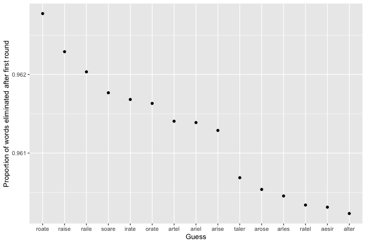
The best word (given knowledge of the set of solutions!) turns out to be “ROATE”, apparently an obsolete variant of “ROTE”4 which is sure to get your table flipped if you play it in Scrabble (though it’s likely to be a bad Scrabble word for the same reasons it’s a good Wordle word!), but eliminates a whopping 96.28% of words on average as the first guess. Just one spot down the line is a much more comfortable word—and one that is in the set of final solutions if you’re looking for that ultimate dopamine hit of getting a hole-in-one—“RAISE”. It lifts you up for a possible win by eliminating 96.23% words on average.
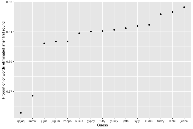
You’re worst off guessing “QAJAQ”, an alternative spelling of “KAYAK”, which only eliminates 55.56% of words after your first try. The first word I recognized on this unfortunate list comes 12 places after “QAJAQ”—covering such ground as “ZOPPO” and “SUSUS”, and is “FUZZY”, which eliminates 62.18% of first words.5 Here are some very bad first guesses:
All this checks out given the letter frequency in the solution set. Summing up the count of each letter in every possible solution and dividing by the total number of letters ($2,315 \times 5$) we see the following table, which shows the top 5 and bottom 5 letters:
| Letter | Relative Frequency |
|---|---|
| e | 0.107 |
| a | 0.085 |
| r | 0.078 |
| o | 0.065 |
| t | 0.063 |
| ... | ... |
| v | 0.013 |
| q | 0.003 |
| x | 0.003 |
| z | 0.003 |
| j | 0.002 |
“ROATE” perfectly combines the top 5 letters, and “QAJAQ” scrapes from the bottom of the barrel.6
I’ll end here and share the code to produce the figures and table at the bottom of the post. Hope this helps your scoreboard, and huge shoutout to Gabriel Gilling. He and I talked through an earlier version of how we would approach this, but I was quite busy at the time we could have worked on it together. He has a really cool idea of taking a Bayesian approach and updating on the way to the final possible answer, which I’ll be sure to link to or add to here if he (or we) get back to it.
results_summary <- sapply(results, function(x)
  mean((length(possible_solutions)-x)/length(possible_solutions))
)

results_summary <- as_tibble(results_summary) %>%
  mutate(word = names(results_summary)) %>%
  relocate(word)

# best guesses

results_summary %>%
  slice_max(value, n = 15) %>%
  ggplot(aes(x = reorder(word, -value), y = value)) +
    geom_point() +
    ylab("Proportion of words eliminated after first round") +
    xlab("Guess")

# worst guesses

results_summary %>%
  slice_min(value, n = 15) %>%
  ggplot(aes(x = reorder(word, value), y = value)) +
  geom_point() +
  ylab("Proportion of words eliminated after first round") +
  xlab("Guess")

# letter frequency

letter_frequency <- lapply(possible_solutions, function(x)
  str_split(x, "", nchar(x))
)

letter_frequency <- unlist(letter_frequency)
letter_frequency <- as_tibble(letter_frequency) %>%
  rename(letter = value) %>%
  group_by(letter) %>%
  summarize(frequency = round(n()/(2315*5), 3)) %>%
  arrange(desc(frequency))
-
Just to not be too self-deprecating—also with much more powerful computers. I could, I think, use Columbia’s computing cluster but I don’t want to risk getting kicked off. ↩
-
I also don’t account for repeated letters in the same way that Wordle handles them in the code as written. ↩
-
This is quite slow (several hours) since there are 12,972 possible guesses and so we have to check 30,030,180 combinations. I’m sure I can make some speed gains here, but this is not my area of expertise, unfortunately. ↩
-
Rote isn’t a very common word in and of itself, either, though it means “the use of memory usually with little intelligence,” or “mechanical or unthinking routine or repetition,” which coincidentally is how my computer felt checking through every possible Wordle answer to find the best first guess. ↩
-
As you can see by comparing to the first figure, there’s a much bigger gap between the worst and second worst guess than between the best and second best guess, although in general, this distribution is fairly equal, with a Gini coefficient of approximately 0.029. ↩
-
This distribution is less equal, with a Gini coefficient of 0.405, comparable to the Gini coefficient of Tanzania. ↩