This week’s Riddler Classic is about a surprising game of dice. Here’s the text of the puzzle, and my solution below.
From Ed Carl comes a surprising game of dice:
We’re playing a game where you have to pick four whole numbers. Then I will roll four fair dice. If any two of the dice add up to any one of the numbers you picked, then you win! Otherwise, you lose.
For example, suppose you picked the numbers 2, 3, 4 and 12, and the four dice came up 1, 2, 4 and 5. Then you’d win, because two of the dice (1 and 2) add up to at least one of the numbers you picked (3).
To maximize your chances of winning, which four numbers should you pick? And what are your chances of winning?
Interestingly for those who play Settlers of Catan and know that 7 is the most likely sum of two die rolls, the winning set of four numbers to pick in this game is 4,6,8, and 10. Your chances of winning with this pick are approximately 97.5%, or $\frac{79}{81}$, reduced from $\frac{1,264}{1,296}$. Let’s walk through how I got to this answer.
We’ll start by enumerating the number of possible rolls the “you” in the puzzle text (let’s call them Ed) can make. This is a question of permutations, since order will matter for the purposes of summing two dice later. We’ll use the gtools library to aid us with combinatorics functions, and ggplot2 for graphs.
library("gtools")
library("ggplot2")

possible_rolls <- permutations(n = 6, r = 4, v = 1:6,
                               repeats.allowed = TRUE)
For four six-sided dice, there are 1,296 possible rolls, so this object yields a matrix with 1,296 rows and 4 columns. We can then (very uninspiringly) check each possible combination (order does not matter since addition is commutative) of two column sums. Since we have 4 columns and have to sum 2 of them, we have ${4 \choose 2} = 6$ possible combinations, each delineated below.
roll_sums <- cbind(possible_rolls[,1] + possible_rolls[,2], # die 1 combined with die 2
                   possible_rolls[,1] + possible_rolls[,3], # die 1 combined with die 3
                   possible_rolls[,1] + possible_rolls[,4], # die 1 combined with die 4
                   possible_rolls[,2] + possible_rolls[,3], # die 2 combined with die 3
                   possible_rolls[,2] + possible_rolls[,4], # die 2 combined with die 4
                   possible_rolls[,3] + possible_rolls[,4]) # die 3 combined with die 4
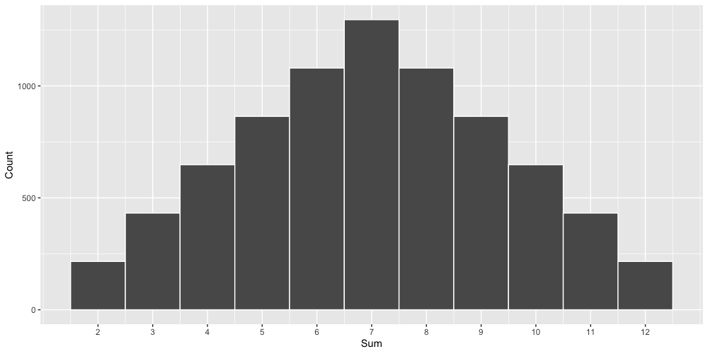
Now roll_sums is a matrix still with 1,296 for each possible row, but with 6 columns to represent each of these sums. Flattening this matrix out into a vector and plotting out the distribution of roll sums, we get the familiar “Catan” distribution, where 7 is the most likely sum of two dice rolls, and the possible sums get progressively less likely as you go out toward the lonely 2 and 12. This makes sense: there are 6 ways to create a sum of 7 from two dice (1 and 6, 2 and 5, 3 and 4, 6 and 1, 2, and 5, 4 and 3) out of 36 total possibilities, and only one way to get to 2 or 12 (1 and 1; 6 and 6, respectively).
roll_sums_df <- data.frame(as.vector(roll_sums))
names(roll_sums_df) <- "sum"

ggplot(roll_sums_df, aes(x = sum)) +
  geom_histogram(bins = 11, color = "white") +
  scale_x_continuous(breaks = 2:12, name = "Sum") +
  scale_y_continuous(name = "Count")
But we’re playing a slightly different game here, so let’s see how things may change. Next, we can check combinations for our possible choices to fare against Ed’s rolls. We should limit our search of four integers to the values from 2 to 12, since there is no possible way for us to win if we select 1 as one of our choices, following the above logic. We also shouldn’t repeat any numbers, since that would just be wasteful!
possible_choices <- combinations(n = 11, r = 4, v = 2:12,
                                 repeats.allowed = FALSE)
This produces a matrix of 330 rows and 4 columns, representing each of our possible choices. Now, for each of our possible choices, let’s check how often two of the dice add up to a number that we selected.
outcomes <- lapply(1:nrow(possible_choices), function(i)
  t(sapply(1:nrow(roll_sums), function(j)
    roll_sums[j,] %in% possible_choices[i,]
  ))
)
This produces a list of length 330 (our total number of possible choices) where each element in the list is how that choice fared for each of Ed’s rolls. For example, our first set of four integers are 2, 3, 4, and 5. Then outcomes[[1]] is a 1,296 by 6 matrix where each row is one of Ed’s dice rolls and each column is TRUE or FALSE if 2, 3, 4, or 5 are included in the row of roll_sums. For Ed’s first roll, which is 1, 1, 1 and 1, the possible sums are all just 2s, and since we selected 2, all the values for this row of outcomes[[1]] will be equal to TRUE. But if the row of roll_sums were say, 2, 2, 6, 2, 6, 6, then the corresponding row for outcomes[[1]] would be TRUE, TRUE, FALSE, TRUE, FALSE, FALSE, since we didn’t select 6 as one of our picks.
So to check if we win for each roll, we now just need to see whether the sum of these rows of outcomes are greater than zero:
results <- sapply(outcomes, function(i)
  apply(i, MARGIN = 1, FUN = sum) > 0
)
Now results is a 1296 by 330 matrix, where rows represent Ed’s rolls and columns are our choices. If we take the mean of each column, we have our final answers, since this will represent the proportion of TRUE values (our wins!). We can also paste our rolls into a single character and sort by win-rate to make everything easier to read.
results_table <- data.frame(sapply(1:nrow(possible_choices), function(i)
  paste0(possible_choices[i,], collapse = ",")
))
names(results_table) <- "choice"
results_table$prop_win <- colMeans(results)
results_table <- results_table[order(results_table$prop_win, decreasing = TRUE),]
| Choice | Win Probability |
|---|---|
| 4, 6, 8, 10 | 0.975 |
| 2, 6, 8, 10 | 0.961 |
| 4, 6, 8, 12 | 0.961 |
| 4, 6, 7, 9 | 0.955 |
| 5, 7, 8, 10 | 0.955 |
| ... | ... |
| 2, 9, 11, 12 | 0.684 |
| 2, 3, 5, 12 | 0.684 |
| 2, 3, 4, 12 | 0.626 |
| 2, 10, 11, 12 | 0.626 |
| 2, 3, 11, 12 | 0.599 |
Surprisingly, the winning pick does not contain a 7, although a 7 is not far behind. Overall, you fare quite well in this game, with even the unsurprisingly bad pick of 2, 3, 11, and 12 giving the player an almost 60% win-rate versus Ed.
comments powered by Disqus