A group of friends and I participate in a mini film club together. Just like a book club we take turns picking a movie and meet to discuss whatever we all watched.
My friends have kindly agreed to share their Letterboxd data with me so that I could discern the exact moment of all our deaths do some simple analyses. My focus is less going to be on any individual person’s film habits and more the descriptives and techniques I’m estimating—as a preview, we’ll see some of our favorite movies, the most controversial movies, a simple recommendation system, each person’s hipsterness ratings, and some text analysis on written reviews. The code itself is fully flexible and can be used with any set of downloaded Letterboxd data files.
For those not in the know, Letterboxd is a social networking site revolving around movies (much like Goodreads is for books): you can log movies you’ve watched, offer ratings and write reviews, comment on other people’s reviews, etc. It’s quite fun and non-toxic which is why I enjoy it.
I’ve done these analyses in R. We’ll start by loading in the packages used:
library("tidyverse") # for general data wrangling
library("gtools") # for permutations
library("rvest") # for webscraping
library("lubridate") # for working with dates
library("tidytext") # for working with text
By placing the unzipped Letterboxd folders into the working directory, we can easily identify the members of the analysis by detecing the folders in the directory which have a regular pattern.
members <- list.files(pattern = "letterboxd-")
This will allow us to create our first data frame, where rows represent User-Film pairs of all the films the users have ever watched. We’ll also go ahead and add some basic information on the number of people who have watched each movie, and highlight those which all users have seen, only one user have seen, and all minus one user have seen. At this point, one might want to edit the User column so the values are more readable instead of the full file names, but in order to keep the code as flexible as possible, I have not done so here.
movies <- lapply(members, function(i)

  read.csv(file = paste0(i, "/watched.csv"))

)

names(movies) <- members

movies <- bind_rows(movies, .id = "User") |>
  rename(URL = Letterboxd.URI) |>
  select(-Date) |>
  mutate(Watched = TRUE)

movies <- movies |>
  group_by(Name, Year, URL) |>
  mutate(N_Watched = sum(!is.na(Watched)),
         All_Watched = N_Watched == length(members),
         All_Minus1_Watched = N_Watched == length(members) - 1,
         Only_1Watched = N_Watched == 1)
We can use pivot_wider to create a wide version of the data, where rows represent a film and each member’s ratings are columns for each individual film. Our group has watched 1,750 unique movies!
movies_wide <- movies |>
  pivot_wider(
    names_from = "User",
    values_from = "Watched",
    names_prefix = "Watched_") |>
  mutate(across(starts_with("Watched"),
                ~ !is.na(.))) |>
  pivot_longer(starts_with("Watched"),
               names_to = "User",
               names_prefix = "Watched_",
               values_to = "Watched") |>
  mutate(Watched = ifelse(Watched, "Watched", "NotWatched")) |>
  group_by(Name, Year, Watched, URL) |>
  summarize(Who = paste0(User, collapse = ", ")) |>
  pivot_wider(names_from = "Watched",
              values_from = "Who",
              names_prefix = "Who_") |>
  mutate(N_Watched = str_count(Who_Watched, ",") + 1,
         All_Watched = N_Watched == length(members),
         All_Minus1_Watched = N_Watched == length(members) - 1,
         Only_1Watched = N_Watched == 1)
Some of the quantities of interest involve using the Letterboxd average ratings for each movie, which are fairly tricky to webscrape. Here’s a function I wrote to get it done. I’ll save it as an .Rdata file to only run that once, since it takes quite a bit to run (notice I use Sys.sleep and the rpois function to generate random breaks between reading in the html of each film’s page). Using each film’s URL as a key, we can join this to the movies and movies_wide data frames.
# Add Letterboxd averages

read_letterboxd_average <- function(url) {

  page <- read_html(url)

  average_rating <- page |>
    html_nodes(xpath = '//meta[@name="twitter:data2"]') |>
    html_attr("content")

  average_rating <- as.numeric(str_replace(average_rating, " out of 5", ""))

  Sys.sleep(min(rpois(n = 1, lambda = 1)+1, 10))

  return(average_rating)

}

letterboxd_averages_raw <- sapply(movies_wide$URL, read_letterboxd_average)
Letterboxd_Rating <- data.frame(letterboxd_averages_raw) |>
  rownames_to_column("URL") |>
  rename(Letterboxd_Rating = letterboxd_averages_raw)

save(Letterboxd_Rating, file = "Letterboxd_Rating.Rdata")

load("Letterboxd_Rating.Rdata")

movies_wide <- left_join(movies_wide, Letterboxd_Rating)

movies <- left_join(movies, movies_wide)
We’re almost done with the data processing steps, we just need to add our own ratings, which is separate from the watched files, since you can watch a movie without rating it.
# Add our ratings

ratings <- lapply(members, function(i)

  read.csv(file = paste0(i, "/ratings.csv"))

)

names(ratings) <- members

ratings <- bind_rows(ratings, .id = "User") |>
  rename(URL = Letterboxd.URI) |>
  select(-Date)

movies <- left_join(movies, ratings)

ratings_wide <- ratings |>
  pivot_wider(
    names_from = "User",
    values_from = "Rating",
    names_prefix = "Rating_") |>
  rowwise() |>
  mutate(Mean_Rating = mean(c_across(starts_with("Rating")), na.rm = TRUE))

movies_wide <- left_join(movies_wide, ratings_wide)
Now we’re ready to go! Let’s start by seeing our favorite movies, by average rating. Of the 27 movies we’ve all seen, our top 5 are Tár, City of God, Jeanne Dielman, 23, quai du Commerce, 1080 Bruxelles, Spirited Away, and Aftersun.
# Best movies we've all watched

best <- movies |>
  group_by(Name, Year, URL) |>
  filter(All_Watched == TRUE) |>
  summarize(rating_mean = mean(Rating, na.rm = TRUE)) |>
  arrange(desc(rating_mean))

best <- left_join(best, movies_wide) |>
  select(Name, Year, rating_mean, starts_with("Rating"), Letterboxd_Rating)

best
How about something a little spicier? We can define our most controversial movies as those with the biggest variance in ratings, both among movies we’ve all watched and more broadly. I’m not going to share these full tables but one of us gave Godzilla vs. Kong a 4-star rating, while another gave it a 1-star rating.
# Most controversial - biggest variance in ratings, among movies we've all watched

controversy <- movies |>
  group_by(Name, Year, URL) |>
  filter(All_Watched == TRUE) |>
  summarize(rating_sd = sd(Rating)) |>
  arrange(desc(rating_sd))

controversy <- left_join(controversy, movies_wide) |>
  select(Name, Year, rating_sd, starts_with("Rating"), Letterboxd_Rating)

controversy

# Most controversial - biggest variance in ratings, all movies

controversy <- movies |>
  group_by(Name, Year, URL) |>
  mutate(rating_sd = sd(Rating, na.rm = TRUE)) |>
  ungroup() |>
  select(Name, Year, rating_sd, Who_Watched) |>
  arrange(desc(rating_sd)) |>
  distinct()

controversy <- left_join(controversy, movies_wide) |>
  select(Name, Year, rating_sd, starts_with("Rating"), Letterboxd_Rating)

controversy
We might also be interested in the “best-missing”—the best movies one of us hasn’t watched, or alternatively any movies only one person has watched, and that single person gave it a 5-star rating:
# Best movies only one of us hasn't watched

best_missing <- movies |>
  group_by(Name) |>
  filter(All_Minus1_Watched == TRUE) |>
  mutate(rating_mean = mean(Rating, na.rm = TRUE),
         rating_sum = sum(Rating, na.rm = TRUE)) |>
  select(Name, Year, rating_mean, rating_sum, Who_NotWatched) |>
  distinct() |>
  arrange(desc(rating_mean), desc(rating_sum)) |>
  select(-rating_sum)

best_missing <- left_join(best_missing, movies_wide) |>
  select(Name, Year, rating_mean, Who_NotWatched, starts_with("Rating"), Letterboxd_Rating)

best_missing

# Best movies only one of us has watched

best_solo <- movies |>
  group_by(Name) |>
  filter(Only_1Watched == TRUE) |>
  select(Name, Year, Rating, Who_Watched) |>
  distinct() |>
  arrange(desc(Rating), Who_Watched)

best_solo |>
  ungroup() |>
  group_by(Who_Watched) |>
  slice_max(Rating, n = 2, with_ties = FALSE)
Next we consider deviations from our ratings with the average Letterboxd rating, both by movie and per user, and most interesting to me, the mean deviation from the mean Letterboxd ratings over all movies a person has rated, which could be construed as that person’s “hipsterness” score. Here we do not take into consideration absolute differences, but of course, you could do that as well.
movies <- movies |>
  mutate(Rating_Diff = Rating - Letterboxd_Rating)

# Biggest outliers by movie

outliers_movies <- movies |>
  group_by(Name, Year) |>
  mutate(mean_rating_diff = mean(Rating_Diff, na.rm = TRUE)) |>
  select(Name, Year, Letterboxd_Rating, mean_rating_diff) |>
  distinct() |>
  arrange(desc(mean_rating_diff))

outliers_movies <- left_join(outliers_movies, movies_wide) |>
  select(Name, Year, mean_rating_diff, Letterboxd_Rating, starts_with("Rating"))

outliers_movies

# Outliers by person for each movie - max

outliers_rater <- movies |>
  group_by(User) |>
  slice_max(Rating_Diff, n = 10) |>
  select(User, Name, Year, Rating, Letterboxd_Rating, Rating_Diff)

outliers_rater <- left_join(outliers_rater, movies_wide) |>
  select(User, Name, Year, Letterboxd_Rating, starts_with("Rating"))

outliers_rater

# Outliers by person for each movie - min

outliers_rater <- movies |>
  group_by(User) |>
  slice_min(Rating_Diff, n = 10) |>
  select(User, Name, Year, Rating, Letterboxd_Rating, Rating_Diff)

outliers_rater <- left_join(outliers_rater, movies_wide) |>
  select(User, Name, Year, Letterboxd_Rating, starts_with("Rating"))

outliers_rater

# By person (hipsterness)

movies |>
  group_by(User) |>
  summarize(mean_rating_diff = mean(Rating_Diff, na.rm = TRUE))
Turning to some slightly more complex procedures, we can see who is most similar to each other in terms of rating movies by calculating cosine similarity ratings for each pair of users. Of course, this is only one similarity metric, you could consider others like Jaccard similarity (with only watched movies or some binarization of the rating), Euclidean distance, and so on.
# Who is the most similar to each other?

combinations_forsimilarity <-
  data.frame(combinations(n = length(members),
                          r = 2,
                          v = members)) |>
  rename(User1 = X1, User2 = X2)

cosine_similarity <- function(x, y) {
  dot_product <- sum(x * y, na.rm = TRUE)
  magnitude_x <- sqrt(sum(x^2, na.rm = TRUE))
  magnitude_y <- sqrt(sum(y^2, na.rm = TRUE))
  similarity <- dot_product / (magnitude_x * magnitude_y)
  return(similarity)
}

combinations_forsimilarity$cosine_similarity <- sapply(1:nrow(combinations_forsimilarity), function(i)

  cosine_similarity(movies_wide[,paste0("Rating_", combinations_forsimilarity[i,]$User1)],
                    movies_wide[,paste0("Rating_", combinations_forsimilarity[i,]$User2)])

)

combinations_forsimilarity
Subsequently this can be the basis of a simple recommendation engine, which takes the combinations_forsimilarity object (which has ${n \choose 2}$ rows, where $n$ is the number of users) and pivots it to the similarity object which just concerns the possible pairings between the target_user and the other users. It then takes the movies data frame and filters it to movies the target_user has not seen, joins the similarity ratings from the other users and creates a weighted rating (if you have many users, you may want to define a threshold by which a user is similar to another) based on the similarity scores. This rating is then transformed to range between 0 and 1 and the output is the list of movies the target_user has not seen sorted by this weighted rating.
# A simple recommendation system: weighted rating

recommendations <- function(target_user) {

  similarity <- combinations_forsimilarity |>
    filter(str_detect(User1, paste0("^", target_user, "$")) |
             str_detect(User2, paste0("^", target_user, "$"))) |>
    pivot_longer(c(User1, User2),
                 values_to = "other_rater") |>
    filter(other_rater != target_user) |>
    mutate(target_user = target_user) |>
    select(-name) |>
    relocate(target_user, other_rater, cosine_similarity)

  output <- movies |>
    filter(str_detect(Who_NotWatched, paste0("^", target_user, "$")) |
             str_detect(Who_NotWatched, paste0(target_user, ",")) |
             str_detect(Who_NotWatched, paste0(target_user, "$"))) |>
    group_by(Name, Year, User) |>
    rename(other_rater = User) |>
    summarize(Rating = Rating)

  output <- left_join(output, similarity)

  output <- output |>
    select(-target_user) |>
    group_by(Name, Year) |>
    summarize(mean_Rating = mean(Rating),
              weighted_Rating = sum(Rating*cosine_similarity))

  min_wt_rating <- min(output$weighted_Rating, na.rm = TRUE)
  max_wt_rating <- max(output$weighted_Rating, na.rm = TRUE)

  output <- output |>
    mutate(weighted_Rating = (weighted_Rating-min_wt_rating)
           /(max_wt_rating-min_wt_rating))

  output <- left_join(output, select(movies_wide,
                                     c("Name", "Year",
                                       starts_with("Rating")))) |>
    arrange(desc(weighted_Rating))

  output <- output[, colSums(is.na(output)) != nrow(output)]

  print(paste0("Printing recommendations for: ", target_user))

  return(output)

}
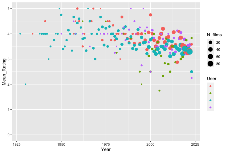
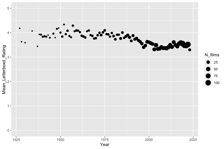
Moving on to more general descriptives, I was curious about average ratings over time, both considering the Letterboxd averages (though note the sample is the set of movies we’ve all seen) and our own ratings:
# Average ratings over time

movies_wide |>
  mutate(Decade = paste0(Year - Year %% 10, "s")) |>
  group_by(Decade) |>
  summarize(Mean_OurRating = mean(Mean_Rating, na.rm = TRUE),
            Mean_LetterboxdRating = mean(Letterboxd_Rating, na.rm = TRUE),
            N_films = n())

movies |>
  group_by(Year, User) |>
  summarize(Mean_Rating = mean(Rating, na.rm = TRUE),
            N_films = n()) |>
  ggplot(aes(x = Year, y = Mean_Rating, color = User, size = N_films)) +
  geom_point() +
  scale_y_continuous(limits = c(0,5))
Next we consider watching behavior. This can be found in the diary files within your Letterboxd data, which contain movies you’ve watched and have recorded the date that you watched it. The most popular single date among our group consisted of 7 movies watched (split across only two users!). Our most popular month consisted of 64 movies logged, and a single user watched 33 movies in a month. The most popular movie months are December and January, not surprising considering the combination of the holidays and the season.
# Read viewing data

diary <- lapply(members, function(i)

  read.csv(file = paste0(i, "/diary.csv"))

)

names(diary) <- members

diary <- bind_rows(diary, .id = "User") |>
  rename(URL = Letterboxd.URI)

# Single most popular watch date

diary |>
  group_by(Watched.Date) |>
  summarize(N_films = n(),
            film_names = paste0(User, " - ", Name, collapse = ", ")) |>
  arrange(desc(N_films))

# Single most popular date by user

diary |>
  group_by(User, Watched.Date) |>
  summarize(N_films = n(),
            film_names = paste0(Name, collapse = ", ")) |>
  arrange(desc(N_films))

# Single most popular watch month

diary |>
  mutate(Watched.Month = floor_date(ymd(Watched.Date), unit = "month")) |>
  group_by(Watched.Month) |>
  summarize(N_films = n(),
            film_names = paste0(User, " - ", Name, collapse = ", ")) |>
  arrange(desc(N_films))

# Single most popular watch month by user

diary |>
  mutate(Watched.Month = floor_date(ymd(Watched.Date), unit = "month")) |>
  group_by(User, Watched.Month) |>
  summarize(N_films = n(),
            film_names = paste0(Name, collapse = ", ")) |>
  arrange(desc(N_films))

# Most popular months not including year

diary |>
  mutate(Month = month(ymd(Watched.Date))) |>
  group_by(Month) |>
  summarize(N_films = n()) |>
  arrange(desc(N_films))

# Most popular months not including year by user

diary |>
  mutate(Month = month(ymd(Watched.Date))) |>
  group_by(Month, User) |>
  summarize(N_films = n()) |>
  arrange(desc(N_films))
Last but not least let’s play around with some text data! We can grab this data from the reviews files. Our longest review was 4,251 characters long.
# Read review data

reviews <- lapply(members, function(i)

  read.csv(file = paste0(i, "/reviews.csv"))

)

names(reviews) <- members

reviews <- bind_rows(reviews, .id = "User")

# Get longest review

reviews <- reviews |>
  mutate(length_of_review = str_length(Review))
Converting this text data to a more friendly form for text analysis allows us to assess our most used words (which aren’t too interesting: movie, film, story, time, love, fun—all suggest we could be a little more clever with our reviews), and do some sentiment analysis. On average our reviews consisted of 56.3% positive words and 43.7% negative words, and this pattern held for each individual user—all of us use more positive words in our reviews than negative words. The two most negative reviews were of Doctor Strange in the Multiverse of Madness and Black Panther: Wakanda Forever, while the most positive review was of Nomadland.
# Clean text data for analysis

reviews_clean <- reviews |>
  mutate(Review_Clean = tolower(Review)) |>
  unnest_tokens(word, Review) |>
  anti_join(stop_words) |>
  select(User, Name, word)

# Most used words

most_used_words <- reviews_clean |>
  group_by(word) |>
  summarize(count = n()) |>
  arrange(desc(count))

most_used_words <- reviews_clean |>
  group_by(word, User) |>
  summarize(count = n()) |>
  arrange(desc(count))

# Reviews sentiment

reviews_sentiment <- reviews_clean |>
  inner_join(get_sentiments("bing"))

reviews_sentiment |>
  group_by(sentiment) |>
  summarize(count = n()/nrow(reviews_sentiment))

reviews_sentiment |>
  group_by(User, sentiment) |>
  summarize(count = n()) |>
  group_by(User) |>
  mutate(prop = count/sum(count))

reviews_sentiment |>
  group_by(Name, User, sentiment) |>
  summarize(count = n()) |>
  group_by(Name, User) |>
  mutate(prop = count/sum(count)) |>
  arrange(desc(count))